A Deep Dive into Monte Carlo Tree Search
2018-05-15
Tagged: machine learning, alphago, software engineering, popular ⭐️
(This was originally a sponsor talk given at PyCon 2018. Unfortunately there is no video.)
A brief history of Go AI
The very first Go AIs used multiple modules to handle each aspect of playing Go - life and death, capturing races, opening theory, endgame theory, and so on. The idea was that by having experts program each module using heuristics, the AI would become an expert in all areas of the game. All that came to a grinding halt with the introduction of Monte Carlo Tree Search (MCTS) around 2008. MCTS is a tree search algorithm that dumped the idea of modules in favor of a generic tree search algorithm that operated in all stages of the game. MCTS AIs still used hand-crafted heuristics to make the tree search more efficient and accurate, but they far outperformed non-MCTS AIs. Go AIs then continued to improve through a mix of algorithmic improvements and better heuristics. In 2016, AlphaGo leapfrogged the best MCTS AIs by replacing some heuristics with deep learning models, and AlphaGoZero in 2018 completely replaced all heuristics with learned models.
AlphaGoZero learns by repeatedly playing against itself, then distilling that experience back into the neural network. This reinforement learning loop is so robust that it can figure out how to play Go starting from random noise. There are two key requirements for this loop to work: that the self-play games represent a higher level of gameplay than the raw neural network output, and that the training process successfully distills this knowledge.
This essay digs into the “how do you reach a higher level of gameplay?” part of the process. Despite replacing all human heuristics, AlphaGoZero still uses tree search algorithms at its core. I hope to convince you that AlphaGoZero’s success is as much due to this algorithm as it is due to machine learning.
Since this was originally a PyCon talk, I’ll also demonstrate the algorithm in Python and show some Python-specific tricks for optimizing the implementation, based on my experience working on MiniGo.
Exploration and Exploitation
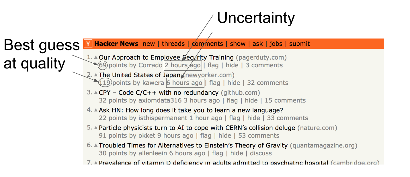
Let’s start by asking a simpler question: how do you rank submissions on Hacker News?

There’s a tension between wanting to show the highest rated submissions (exploitation), but also wanting to discover the good submissions among the firehose of new submissions (exploration). If you show the highest rated submissions only, you’ll get a rich-get-richer effect where you never discover new stories.
The canonical solution to this problem is to use Upper Confidence Bounds.

The idea is simple. Instead of ranking according to estimated rating, you add a bonus based on how uncertain you are about the rating to yield an upper confidence bound. In this example, the top submission on HN has fewer upvotes than the second rank submission, but it’s also newer. So it gets a bigger uncertainty bonus. The uncertainty bonus fades over time, and that submission will fall in ranking unless it can prove its worth with more upvotes.
This is an instance of the Multi Armed Bandit problem and has a pretty extensive literature if you want to learn more.
UCT = Upper Confidence bounds applied to Trees
So how does this help us understand AlphaGoZero? Playing a game has a lot in common with the multi-armed bandit problem: when reading into a game variation, you want to balance between playing the strongest known response, and exploring new variations that could turn out to be good moves. So it makes sense that we can reuse the UCB idea.
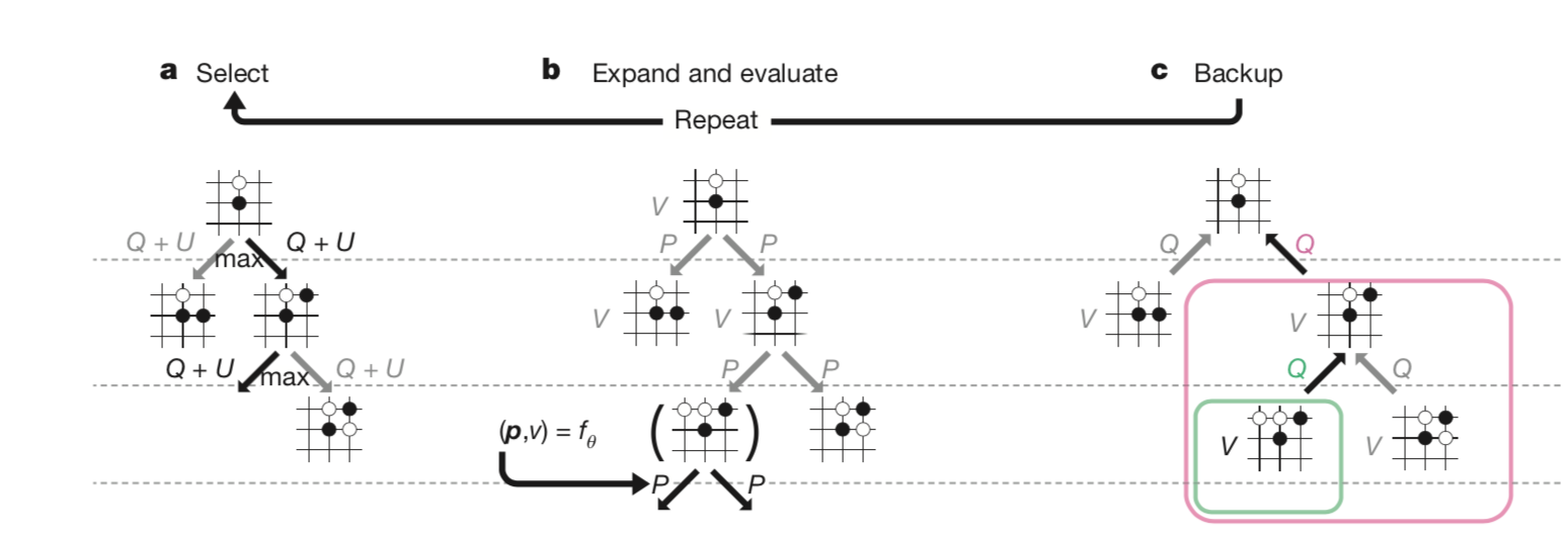
This figure from the AlphaGoZero paper lays out the steps.

First, we select a new variation to evaluate. This is done by recursively picking the move that has highest Q+U score until we reach a variation that we have not yet evaluated.
Next, we pass the variation to a neural network for evaluation. We get back two things: an array of probabilities, indicating the net’s preference for each followup move, and a position evaluation.
Normally, with a UCB algorithm, all of the options have equal uncertainty. But in this case, the neural network gives us an array of probabilities indicating which followup moves are plausible. Those moves get higher uncertainty bonuses, ensuring that our tree search looks at those moves first.
The position evaluation can be returned in one of two ways: in an absolute sense, where 1 = black wins, -1 = white wins, or in a relative sense, where 1 = player to play is winning; -1 player to play is losing. Either way, we’ll have to be careful about what we mean by “maximum Q score”; we want to reorient Q so that we’re always picking the best move for Black or White when it’s their turn. The Python implementation I show will use the absolute sense.
As a historical note, the first MCTS Go AIs attempted to evaluate positions by randomly playing them out to the end and scoring the finished game. This is where the Monte Carlo in MCTS comes from. But now that we no longer do the MC part of MCTS, MCTS is somewhat of a misnomer. So the proper name should really just be UCT search.
Finally, we walk back up the game tree, averaging in the the position evaluation at each node along the way. The net result is that a node’s Q score will be the average of its subtree’s evaluations.
This process is repeated however long we’d like; each additional search fleshes out the game tree with one new variation. UCT search is a neat algorithm because it can be stopped at any time with no wasted work, and unlike the minimax algorithm, UCT search is flexible enough to explore widely or deeply as it sees fit. For deep, narrow sequences like reading ladders, this flexibility is important.
A basic implementation in Python
Let’s start at the top. The following code is a straightforward translation of each step discussed above.
def UCT_search(game_state, num_reads):
    root = UCTNode(game_state)
    for _ in range(num_reads):
        leaf = root.select_leaf()
        child_priors, value_estimate = NeuralNet.evaluate(leaf.game_state)
        leaf.expand(child_priors)
        leaf.backup(value_estimate)
    return max(root.children.items(),
               key=lambda item: item[1].number_visits)
The node class is also pretty straightforward: it has references to the game state it represents, pointers to its parent and children nodes, and a running tally of evaluation results.
class UCTNode():
    def __init__(self, game_state, parent=None, prior=0):
        self.game_state = game_state
        self.is_expanded = False
        self.parent = parent  # Optional[UCTNode]
        self.children = {}  # Dict[move, UCTNode]
        self.prior = prior  # float
        self.total_value = 0  # float
        self.number_visits = 0  # int
Step 1 (selection) occurs by repeatedly selecting the child node with the largest Q + U score. Q is calculated as the average of all evaluations. U is a bit more complex; the important part of the U formula is that it has the number of visits in the denominator, ensuring that as a node is repeatedly visited, its uncertainty bonus shrinks inversely proportional to the number of visits.
def Q(self) -> float:
    return self.total_value / (1 + self.number_visits)

def U(self) -> float:
    return (math.sqrt(self.parent.number_visits)
        * self.prior / (1 + self.number_visits))

def best_child(self) -> UCTNode:
    return max(self.children.values(),
               key=lambda node: node.Q() + node.U())

def select_leaf(self) -> UCTNode:
    current = self
    while current.is_expanded:
        current = current.best_child()
    return current
Step 2 (expansion) is pretty straightforward: mark the node as expanded and create child nodes to be explored on subsequent iterations.
def expand(self, child_priors):
    self.is_expanded = True
    for move, prior in enumerate(child_priors):
        self.add_child(move, prior)

def add_child(self, move, prior):
    self.children[move] = UCTNode(
        self.game_state.play(move), parent=self, prior=prior)
Step 3 (backup) is also mostly straightforward: increment visit counts and add the value estimation to the tally. The one tricky step is that the value estimate must be inverted, depending on whose turn it is to play. This ensures that the “max” Q value is in fact the best Q from the perspective of the player whose turn it is to play.
def backup(self, value_estimate):
    current = self
    while current.parent is not None:
        current.number_visits += 1
        current.total_value += (value_estimate *
            self.game_state.to_play)
        current = current.parent
And there we have it - a barebones implementation of UCT search in about 50 lines of Python.
Unfortunately, the basic implementation performs rather poorly. When executed with \(10^4\) iterations of search, this implementation takes 30 seconds to execute, consuming 2 GB of memory. Given that many Go engines commonly execute \(10^5\) or even \(10^6\) searches before selecting a move, this is rather poor performance. This implementation has stubbed out the gameplay logic and the neural network execution, so the time and space shown here represents overhead due purely to search.
What went wrong? Do we just blame Python for being slow?
Well, kind of. The problem with the basic implementation is that we instantiate hundreds of UCTNode objects, solely for the purpose of iterating over them and doing some arithmetic on each node to calculate Q and U. Each individual operation is fast, but when we execute thousands of Python operations (attribute access, addition, multiplication, comparisons) to complete just one child node selection, the whole thing inevitably becomes slow.
Optimizing for performance using NumPy
One strategy for minimizing the number of Python operations is to get more bang for the buck, by using NumPy.
The way NumPy works is by executing the same operation across an entire vector or matrix of elements. Adding two vectors in NumPy only requires one NumPy operation, regardless of the size of the vectors. NumPy will then delegate the actual computation to an implementation done in C or sometimes even Fortran.
>>> nodes = [(0.7, 0.1), (0.3, 0.3), (0.4, 0.2)]
>>> q_plus_u = [_1 + _2 for _1, _2 in nodes]
>>> q_plus_u
[0.8, 0.6, 0.6]
>>> max(range(len(q_plus_u)), key=lambda i: q_plus_u[i])
0

>>> import numpy as np
>>> q = np.array([0.7, 0.3, 0.4])
>>> u = np.array([0.1, 0.3, 0.2])
>>> q_plus_u = q + u
>>> q_plus_u
array([0.8, 0.6, 0.6])
>>> np.argmax(q_plus_u)
0
This switch in coding style is an instance of the array of structs vs struct of arrays idea which appears over and over in various contexts. Row vs. column oriented databases is another place this idea pops up.
So how do we integrate NumPy into our basic implementation? The first step is to switch perspectives; instead of having each node knowing about its own Q/U statistics, each node now knows about the Q/U statistics of its children.
class UCTNode():
    def __init__(self, game_state,
                 move, parent=None):
        self.game_state = game_state
        self.move = move
        self.is_expanded = False
        self.parent = parent  # Optional[UCTNode]
        self.children = {}  # Dict[move, UCTNode]
        self.child_priors = np.zeros(
            [362], dtype=np.float32)
        self.child_total_value = np.zeros(
            [362], dtype=np.float32)
        self.child_number_visits = np.zeros(
            [362], dtype=np.float32)
This already results in huge memory savings. Now, we only add child nodes when exploring a new variation, rather than eagerly expanding all child nodes. The result is that we instantiate a hundred times fewer UCTNode objects, so the overhead there is gone. NumPy is also great about packing in the bytes - the memory consumption of a numpy array containing 362 float32 values is not much more than 362 * 4 bytes. The python equivalent would have a PyObject wrapper around every float, resulting in a much larger memory footprint.
Now that each node no longer knows about its own statistics, we create aliases for a node’s statistics by using property getters and setters. These allow us to transparently proxy these properties to the relevant entry in the parents’ child arrays.
@property
def number_visits(self):
    return self.parent.child_number_visits[self.move]

@number_visits.setter
def number_visits(self, value):
    self.parent.child_number_visits[self.move] = value

@property
def total_value(self):
    return self.parent.child_total_value[self.move]

@total_value.setter
def total_value(self, value):
    self.parent.child_total_value[self.move] = value
These aliases work for both reading and writing values - as a result,
the rest of the code stays about the same! There is no sacrifice in code
clarity to accomodate the numpy perspective switch. As an example, see
the new implementation of child_U which uses the property
self.number_visits.
def child_Q(self):
    return self.child_total_value / (1 + self.child_number_visits)

def child_U(self):
    return math.sqrt(self.number_visits) * (
        self.child_priors / (1 + self.child_number_visits))

def best_child(self):
    return np.argmax(self.child_Q() + self.child_U())
They look identical to the original declarations. The only difference is that previously, each arithmetic operation only worked on one Python float, whereas now, they operate over entire arrays.
How does this optimized implementation perform?
When doing the same \(10^4\) iterations of search, this implementation runs in 90 MB of memory (a 20x improvement) and in 0.8 seconds (a 40x improvement). In fact, the memory improvement is understated, as 20MB of the 90MB footprint is due to the Python VM and imported numpy modules. If you let the NumPy implementation run for the full 30 seconds that the previous implementation ran for, it completes 300,000 iterations while consuming 2GB of memory - so 30x more iterations in the same time and space.
The performance wins here come from eliminating thousands of repetitive Python operations and unnecessary objects, and replacing them with a handful of NumPy operations operating on compact arrays of floats. This requires a perspective shift in the code, but with judicious use of @property decorators, readability is preserved.
Other components of a UCT implementation
The code I’ve shown so far is pretty barebones. A UCT implementation must handle these additional details:
- Disallowing illegal moves.
- Detecting when a variation represents a completed game, and scoring according to the actual rules, rather than the network’s approximation.
- Imposing a move limit to prevent arbitrarily long games
Additionally, the following optimizations can be considered:
- Subtree reuse
- Pondering (thinking during the opponent’s time)
- Parent-Q initialization
- Tuning relative weights of Q, U
- Virtual Losses
Of these optimizations, one of them is particularly simple yet incredibly important to AlphaGoZero’s operation - virtual losses.
Virtual losses
Until now, I’ve been talking about the Python parts of UCT search. But there’s also a neural network to consider, and one of the things we know about the GPUs that execute the calculations is that GPUs like big batches. Instead of passing in just one variation at a time, it would be preferable to pass in 8 or 16 variations at once.
Unfortunately, the algorithms as implemented above are 100%
deterministic, meaning that repeated calls to select_leaf()
will return the same variation each time!
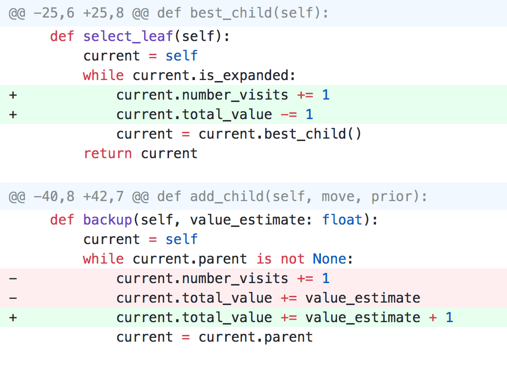
To fix this requires five changed lines:

This change causes select_leaf to pretend as if it
already knew the evaluation results (a loss) and apply it to every node
it passes through. This causes subsequent calls to
select_leaf to avoid this exact variation, instead picking
the second most interesting variation. After submitting a batch of
multiple variations to the neural network, the virtual loss is reverted
and replaced with the actual evaluation.
(The 5 line change is a bit of an oversimplification; implementing virtual losses requires handling a bunch of edge cases, like “what if the same leaf gets selected twice despite the virtual loss” and “tree consists of one root node”)
The overall scaling made possible by virtual losses is something like 50x. This number comes from significantly increased throughput on the GPU (say, 8x throughput). Also, now that leaf selection and leaf evaluation have been completely decoupled, you can actually scale up the number of GPUs - the match version of AlphaGoZero actually had 4 TPUs cooperating on searching a single game tree. So that’s another 4x. And finally, since the CPU and GPU/TPU are now executing in parallel instead of in series, you can think of it as another 2x speedup.
Summary
I’ve shown how and why UCT search works, a basic Python implementation as well as an optimized implementation using NumPy, and another optimization that gives smoother integration of UCT search with multiple GPUs/TPUs.
Hopefully you’ll agree with me that UCT search is a significant contribution to AlphaGoZero’s reinforcement learning loop.
The example code shown here is available in a git repo. You can see
the productionized version with all the optimizations in the Minigo codebase - see
mcts.py and strategies.py in particular.