How to shuffle in TensorFlow
2018-04-04
Tagged: software engineering, machine learning, popular ⭐️
Introduction
If you’ve ever played Magic: The Gathering or other card games where card decks routinely exceed the size of your hands, you’ve probably wondered: How the heck am I supposed to shuffle this thing? How would I even know if I were shuffling properly?
As it turns out, there are similar problems in machine learning, where training datasets routinely exceed the size of your machine’s memory. Shuffling here is very important; imagine you (the model) are swimming through the ocean (the data) trying to predict an average water temperature (the outcome). You won’t really be able to give a good answer because the ocean is not well shuffled.
In practice, insufficiently shuffled datasets tend to manifest as spiky loss curves: the loss drops very low as the model overfits to one type of data, and then when the data changes style, the loss spikes back up to random chance levels, and then steadily overfits again.
TensorFlow provides a rather simple api for shuffling data streams:
Dataset.shuffle(buffer_size).
Let’s try to understand what’s happening under the hood as you mess with
the buffer_size parameter.
Visualizing shuffledness
The seemingly simple way to measure shuffledness would be to come up
with some measure of shuffledness, and compare this number between
different invocations of dataset.shuffle(). But I spent a
while trying to come up with an equation that could measure shuffledness
and came up blank. As it turns out, people have come up with complicated
test suites like Diehard or Crush to try to measure
the quality of pseudorandom number generators, so it suffices to say
that it’s a hard problem.
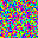
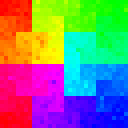
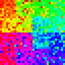
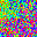
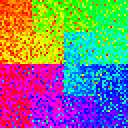
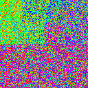
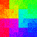
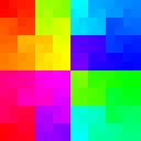
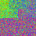
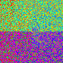
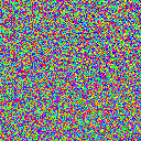
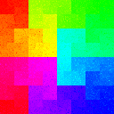
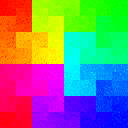
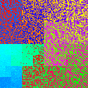
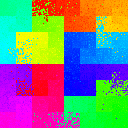
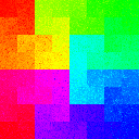
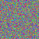
Instead, I decided I’d try to visualize the data directly, in a way that would highlight unshuffled patches of data.
To do this, we use the Hilbert Curve, a space-filling fractal that can take a 1D sequence of data and shove it into a 2D space, in a way that if two points are close to each other in the 1D sequence, then they’ll be close in 2D space.

|

|

|

|

|
Each element of the list then gets mapped to a color on the color wheel.

Exploring shuffler configurations
Basic shuffling
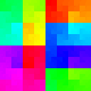
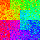
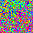
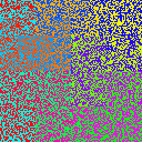
Let’s start with the simplest shuffle. We’ll start with a dataset and stream it through a shuffler of varying size. In the following table, we have datasets of size , and shufflers of buffer size 0%, 1%, 10%, 50%, and 100% of the data size.
buffer_size = int(ratio * len(dataset)) or 1
dataset.shuffle(buffer_size=buffer_size)| Buffer size ratio | ||||||
|---|---|---|---|---|---|---|
| # data | 0 | 0.01 | 0.1 | 0.5 | 1 | |
| 1024 |
|
|
|
|
|
|
| 4096 |

|

|
|
|
|
|
| 16384 |

|

|
|
|
|
|
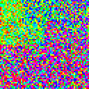
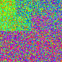
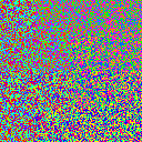
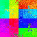
As it turns out, using a simple dataset.shuffle() is
good enough to scramble the exact ordering of the data when making
multiple passes over your data, but it’s not good for much else. It
completely fails to destroy any large-scale correlations in your
data.
Another interesting discovery here is that the buffer size ratio [buffer size / dataset size] appears to be scale-free, meaning that even as we scaled up to a much larger dataset, the qualitative shuffling behavior would remain unchanged if the buffer size ratio stays the same. This gives us the confidence to say that our toy examples here will generalize to real datasets.
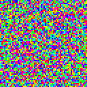
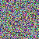
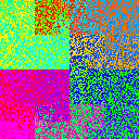
Chained shufflers
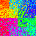
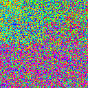
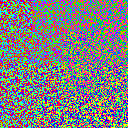
The next thought I had was whether you could do any better by chaining multiple .shuffle() calls in a row. To be fair, I kept the memory budget constant, so if I used 4 chained shuffle calls, each shuffle call would get 1/4 the buffer size. In the following table, we have 1, 2, or 4 chained shufflers, with buffer size ratios of 0%, 1%, 10%, and 50%. All graphs from here on use a dataset size of .
buffer_size = int(ratio * len(dataset) / num_chained) or 1
for i in range(num_chained):
dataset = dataset.shuffle(buffer_size=buffer_size)| # chained shufflers | ||||
|---|---|---|---|---|
| buffer size | 1 | 2 | 4 | |
| 0 |

|

|

|
|
| 0.01 |

|

|

|
|
| 0.1 |
|
|
|
|
| 0.5 |
|
|
|
|
The discovery here is that chaining shufflers results in worse performance than just using one big shuffler.
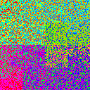
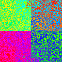
Sharded shuffling
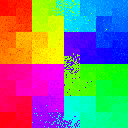
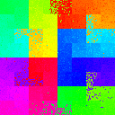
It seems, then, that we need some way to create large-scale movement of data. The simplest way to do this is to shard your data into multiple smaller chunks. In fact, if you’re working on very large datasets, chances are your data is already sharded to begin with. In the following table, we have 1, 2, 4, or 8 shards of data, with buffer size ratios of 0%, 1%, 10%, and 50%. The order of shards is randomized.
dataset = shard_dataset.interleave(
    cycle_length=1, block_length=1)
buffer_size = int(ratio * len(dataset))
dataset = dataset.shuffle(buffer_size=buffer_size)| number of shards | |||||
|---|---|---|---|---|---|
| buffer size | 1 | 2 | 4 | 8 | |
| 0 |

|

|
|
|
|
| 0.01 |

|

|
|

|
|
| 0.1 |
|
|
|
|
|
| 0.5 |
|
|
|
|
|
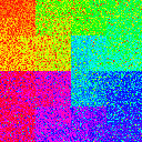
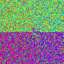
Parallel-read sharded shuffling
The last table didn’t look particularly great, but wait till you see this one. A logical next step with sharded data is to read multiple shards concurrently. Luckily, TensorFlow’s dataset.interleave API makes this really easy to do.
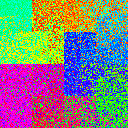
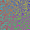
The following table has 1, 2, 4, 8 shards, with 1, 2, 4, 8 of those shards being read in parallel. All graphs from here on use a buffer size ratio of 1%.
shard_dataset = tf.data.Dataset.from_tensor_slices(shards)
dataset = shard_dataset.interleave(lambda x: x
    cycle_length=parallel_reads, block_length=1)
buffer_size = int(ratio * len(dataset))
dataset = dataset.shuffle(buffer_size=buffer_size)| shards read in parallel | |||||
|---|---|---|---|---|---|
| # shards | 1 | 2 | 4 | 8 | |
| 1 |

|
||||
| 2 |

|
|
|||
| 4 |

|
|
|
||
| 8 |
|
|
|
|
|
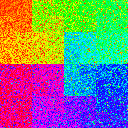
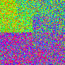
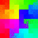
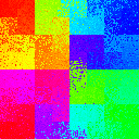
We’re starting to see some interesting things, namely that when #shards = #parallel reads, we get some pretty darn good shuffling. There are still a few issues: because all the shards are exactly the same size, we see stark boundaries when a set of shards are completed simultaneously. Additionally, because each shard is unshuffled, we see a slowly changing gradient across the image as each shard is read from front to back in parallel. This pattern is most apparent in the 2, 2 and 4, 4 table entries.
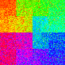
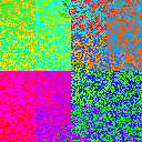
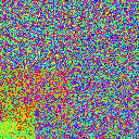
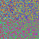
Parallel-read sharded shuffling, with shard size jittering
Next, I tried jittering the shard sizes to try and fix the shard boundary issue. The following table is identical to the previous one, except that shard sizes range from 0.75~1.5x of the previous table’s shards.
| shards read in parallel | |||||
|---|---|---|---|---|---|
| # shards | 1 | 2 | 4 | 8 | |
| 1 |
|
||||
| 2 |
|
|
|||
| 4 |
|
|
|
||
| 8 |
|
|
|
|
|
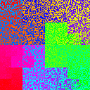
This table doesn’t look that great; the big blobs of color occur because whichever shard is the biggest, ends up being the only shard left over at the end. We’ve succeeded in smearing the sharp shard boundaries we saw in the previous table, but jittering has not solved the large-scale gradient in color.
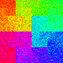
Multi-stage shuffling
So now we’re back to reading in parallel from many shards. How might we shuffle the data within each shard? Well, if sharding the original dataset results in shards that fit in memory, then we can just shuffle them - simple enough. But if not, then we can actually just recursively shard our files until they get small enough to fit in memory! The number of sharding stages would then grow as log(N).
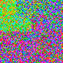
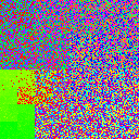
Here’s what two-stage shuffling looks like. Each stage is shuffled with the same parameters - number of shards, number of shards read in parallel, and buffer size.
| shards read in parallel | |||||
|---|---|---|---|---|---|
| # shards | 1 | 2 | 4 | 8 | |
| 1 |

|
||||
| 2 |
|
|
|||
| 4 |
|
|
|
||
| 8 |
|
|
|
|
|
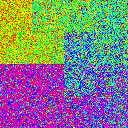
This table shows strictly superior results to our original parallel read table.
Conclusions
I’ve shown here a setup of recursive shuffling that should pretty reliably shuffle data that is perfectly sorted. In practice, your datasets will have different kinds of sortedness at different scales. The important thing is to be able to break correlations at each of these scales.
To summarize:
- A single streaming shuffler can only remove correlations that are closer than its buffer size.
- Shard your data and read in parallel.
- Shards should themselves be free of large-scale correlations.
- For really big datasets, use multiple passes of shuffling.
All code can be found on Github.