Explaining Backpropagation in Neural Networks using Pascal's Triangle
Originally posted 2016-05-19
Tagged: machine learning, computer science
Obligatory disclaimer: all opinions are mine and not of my employer
Neural networks are getting a lot of press lately. I was personally convinced that there’s something very important going on after AlphaGo trounced Lee Sedol in a five game match.
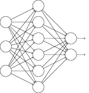
A neural network is simply a network of “neurons”. A neuron takes multiple inputs, and gives one output. A network is created by layering these neurons, so that one layer of neurons operates on the output from the previous layer of neurons. The first layer of this network consists of fake neurons that emits the input, and the final layer of neurons emits the result.

In one of the simpler neural networks (a multilayer perceptron), a neuron takes a weighted combination of its inputs, applies some function (typically a sigmoid function), and emits the result. The parameters of this neural network are the weights that each neuron associates with each of its inputs.
Training a multilayer perceptron is the difficult part: it’s not obvious what weights we should use. There’s quite a few weights to simultaneously optimize; one for each connection between neurons. To start, we can define a cost function that calculates how inaccurate our current network’s output is, and then attempt to optimize all the weights to minimize this cost function. Luckily, optimizing multiple variables simultaneously is a problem that calculus has solved a long time ago. The solution is to calculate the gradient: an array of partial derivatives indicating how the final output’s accuracy depends on each of the weights. If changing a certain weight would result in a dramatic increase in accuracy, then we should change that weight a lot. If changing a certain weight would not alter the accuracy, then we shouldn’t change that weight. And if changing a certain weight would decrease the accuracy, we should change that weight in the opposite direction. Then, perturb your current weights in the ratio prescribed by the computed gradient. This is called gradient descent. Rinse and repeat, and we will have arrived at a locally optimal set of weights.
The issue is that computing partial derivatives with respect to a weight is potentially expensive. If we know nothing about a function \(f\) other than how to compute \(f(x)\) given some \(x\), then approximating its derivative at a given location \(x\) is doable but slow: plug in \(x\) and \(x+h\) for some small \(h\), then compute \((f(x+h) - f(x))/h\). Following this approach, to compute a partial derivative with respect to a weight, you would have to perturb that weight, and then re-execute the entire neural network to see how the output changes. If there are N connections between neurons in your network, a single iteration of gradient descent would cost N executions of your network.
We can do better than that. We like to treat neural networks as black boxes, but we aren’t entirely clueless about the inner workings. In vectorized form, a neural network is described as follows:
\[a^l = \sigma(w^la^{l-1} + b^l)\]
Here, \(a^l\) represents the output of the \(l\)-th layer of neurons; \(w^l\) is a matrix such that \(w_{jk}\) represents the weight given by neuron \(j\) in layer \(l\) to its input neuron \(k\) from layer \(l-1\); \(b^l\) is the bias or offset; and \(\sigma\) is the sigmoid function, \(1/(1 + e^x)\). Each layer’s outputs can be directly plugged into the next layer.
Since the equations describing the neurons are known, one could theoretically write an explicit equation for the cost function, and then take partial derivatives with respect to each of the weights. This ends up in a mess. Since each neuron depends on all of the outputs from the previous layer, we end up with a mess of chain rules: the dependence of the cost function on any given neuron is the sum over all possible paths from that neuron to the output, with each summand being a product of chain rule partial derivatives - the dependence of each neuron on the previous neuron in the path. The last layer of neurons ends up with a very simple derivative (since it is directly related to the cost function), but the first layer of neurons ends up with a monstrously complicated derivative.
Backpropagation is a fancy mathematical trick that simplifies the computation of all of these partial derivatives. It works by reusing computations from one layer to compute the previous layer, starting from the easiest-to-compute last layer and ending with the first. (Hence, “back”-propagation)
I’ll explain with an analogy to another problem.

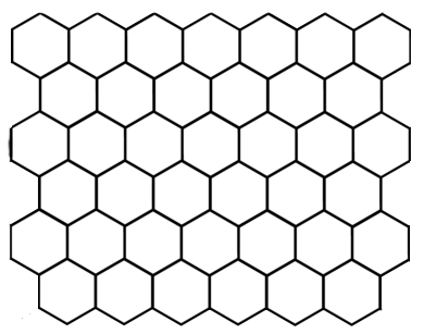
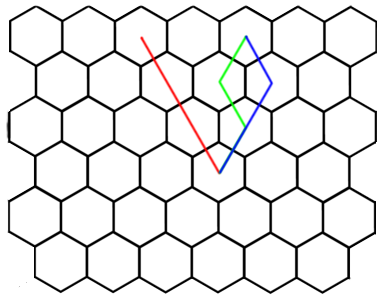
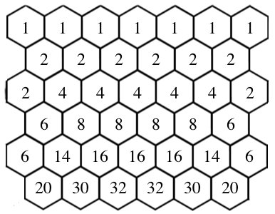
The problem is simple: fill in this grid. The number to be placed in a given cell is the number of distinct paths from the top level of cells to that cell, with paths only allowed diagonally downwards.

Like our partial derivatives problem, each cell has many pathways leading to it, all of which must be accounted for. The top layer of cells is easy to compute, as the paths are trivial (all have 1 path). But the bottom layer of cells is more difficult to compute, with many such paths
There’s a simple trick that makes this problem quite easy. Once we’ve computed a layer of this grid, we can reuse that layer to compute the next layer. This is because you can only arrive at a cell in two ways: from the upper left or upper right. Like in Pascal’s triangle, we can then fill in the entries of this grid.

This is a classic example of dynamic programming: reusing the results of a smaller problem to solve slightly bigger problems. Our partial derivatives problem can be solved in the same way. The last layer of neurons can easily be computed, and with those results, the second-to-last layer of neurons can be more easily computed. Instead of worrying about all possible paths from a neuron to the final layer, just worry about the paths from a neuron to the next layer. The knowledge of all possible paths beyond that layer is already encapsulated in the value we’ve calculated. Working backwards, we can fill in all of the partial derivatives, layer by layer.
To learn more, I recommend Neural Networks and Deep Learning, an online textbook.